AusTraits use case
Summary:
The team at AusTraits have compiled data on plant traits for nearly 500 traits across more than 30,000 taxa. Bringing together extremely heterogeneous data into one database with a unified ontology has impressed many ecologists and we are now excited that these rich data are available for download through the ‘austraits’ R package. The EcoCommons team is looking forward to finalising a direct connection to the AusTraits’ data through an API connection, which is already being used to display summary trait values on the Atlas of Living Australia species factsheets, as part of their Biodiversity Information Explorer platform. Here we demonstrate how we used the AusTraits’ R package to download and filter appropriate data. We also provide some examples of how one might run an analysis on EcoCommons which predicts how a trait varies spatially in both R and in EcoCommons dashboard tools, or how a trait might relate to another grouping variable in a simple GLMM in R. The examples we are providing are scientifically SILLY, but they demonstrate how to access AusTraits’ data and provide demonstrations of the kinds of things you can do on EcoCommons.
By – Dr Rob Clemens, Phil Trovato, Dr David Coleman, & Dr Elizabeth Wenk
An overview of AusTraits data, accessing or filtering those data, using the ‘austraits’ R-package, and examples of analyses in R with spatial data
Introduction:
There is growing interest in the utility of plant trait data (Bradshaw et al. 2011, Myers-Smith et al. 2018, Hagen et al. 2023). The work by the AusTraits’ team to harmonise Australian plant trait data into one database started in 2016 but was only released publicly in 2021 (Falster et al. 2021). With already 44 citations indicated by Google scholar to their 2021 paper, and over 500 data contributors, the popularity of these data is clearly high.
There is a vast array of analyses that could be conducted using the AusTraits data. Here we focus on a couple of examples that leverage the extensive quantities of spatial data available on EcoCommons to predict how a species trait varies spatially using a generalised linear model (GLM) and a generalized additive model (GAM). Currently, this kind of analysis draws upon a relatively small subset of available data. First, there are relatively few AusTraits data that include latitude and longitude. Second, the available predictor variables in these examples are limited to those represented by spatial grids (rasters). We then also provide one simple generalized linear mixed model (GLMM) example of how to examine how a trait varies based on another variable that can be grouped.
Again, these demonstrations do not highlight good science, they simply show examples of the kinds of data extraction, filtering and subsequent analysis that can be done.
Methods:
There are currently over 1.2 million trait measurement records in the AusTraits data (Table 1), and the “austraits” R package allows for easy access, sub-setting, summarising and wrangling of those data. The example R code for this use case shows a number of different ways to summarise the available data and then subset the data to those records that are of interest.
In this use case, we focussed on those data with latitude and longitude associated with the trait measurement so that we could make spatial predictions of how traits vary. The subset of records with latitude and longitude recorded included over 300,000 records. If we look at the number of continuous traits that were measured for each combination of trait and species that also recorded latitude and longitude and had a minimum of 30 or more records we find that there are over 1000 individual trait by taxa combinations that have between 30 and 500+ records (Figure 1).
Table 1. The ‘summarise_austraits’ function in the R package provides an overview of the number of records, datasets and taxa available for each of 464 traits. Below is a summary of records for a small subset of traits.
| trait_name | # records | # datasets | # taxa |
| plant_growth_form | 136449 | 96 | 32851 |
| plant_height | 40852 | 68 | 17711 |
| leaf_length | 40673 | 43 | 14619 |
| seed_dry_mass | 39683 | 49 | 9985 |
| leaf_width | 39668 | 45 | 14149 |
| fruit_fleshiness | 31295 | 14 | 21207 |
| flowering_time | 30939 | 31 | 18104 |
| fruit_type | 29138 | 11 | 20801 |
| stem_growth_habit | 24478 | 22 | 14744 |
| leaf_area | 22470 | 91 | 4841 |
| seed_length | 20025 | 33 | 7724 |
| fire_response | 19500 | 29 | 10522 |
| leaf_compoundness | 18964 | 27 | 13748 |
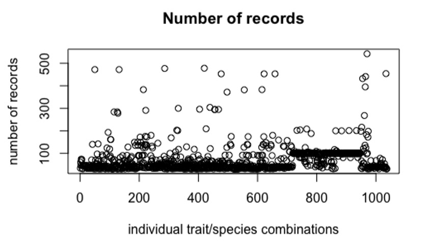
Figure 1. The number of AusTraits records for each of 1,037 individual species & trait combinations where both latitude and longitude were recorded and there were at least 30 records.
Many of the lines of code in our example use case simply highlight a variety of ways to summarise and subset data. Lines 74 through 107 demonstrate how a ‘for loop’ in R can be used to generate a table where the number of records is totalled for each trait with a minimum of 10 records with unique spatial coordinates for each trait by species combination. Lines 123 to 194 show a similar example of subsetting variables to get the subset of leaf area trait measurements for species that had those measurements taken at a minimum of 10 unique spatial locations. Lines 204 through 241 highlight a number of ways to generate different kinds of summary tables. Line 255 through line 316 show a couple of ways to get a resulting table with all the ‘leaf area’ measurements taken from the species Pittosporum undulatum where the average of values was taken at locations with multiple measurements. Lines 325 through 342 show how to format the data from the Pittosporum undulatum measurements and then download two spatial predictors, average annual rainfall and average annual precipitation (Figure 2). Any spatial layers could be used, and it would make sense to restrict the extent of predictions to areas where Pittosporum undulatum is known to occur.
Line 349 creates a spatial points layer from the data table, and lines 354 though 358 then extracts the values of temperature and precipitation at those locations and combine them into the data table with leaf area trait values. Line 361 then show a simple way to generate a correlation matrix between selected variables (Figure 3). Note the high correlation between rainfall and temperature in this example highlight another reason we would not use this example in any serious scientific analysis. Generally, high correlations between predictor variables result in multicollinearity which often muddies the interpretation of coefficients estimated from statistical models.
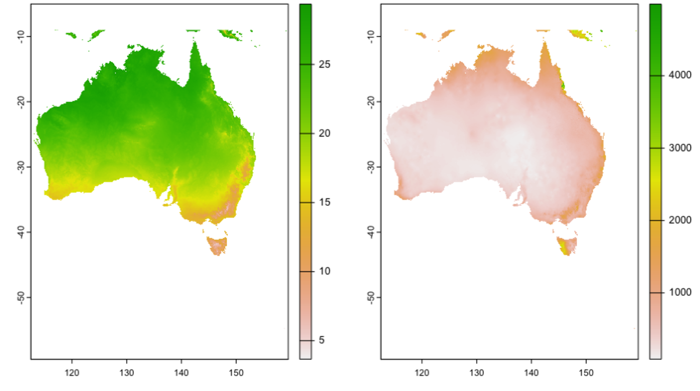
Figure 2. The geospatial data used in subsequent models including, left = mean annual temperature, right = mean annual rainfall.
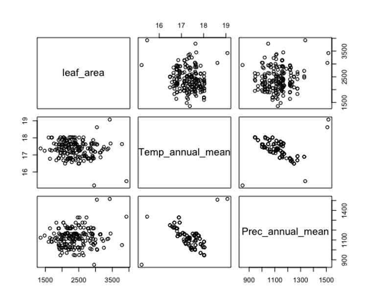
Figure 3. A simple correlation matrix showing the pattern of correlations between the leaf area response variable and the explanatory variables of mean annual temperature and mean annual rainfall.
Using the latest table of data, we first fit a simple generalised linear model (GLM), and then used that model to predict how leaf area might vary spatially (Lines 368 – 371).
Using the ‘mgcv’ package we then attempted to fit a generalised additive model (GAM) to capture non-linear relationships between Pittosporum undulatum leaf area, and annual precipitation or temperature. There was insuffient v variation in the available data to run a GAM, so for demonstration purposes, we added the sequential row id number to both predictors (lines 380 – 381). We then got a GAM to run with invented data and predicted how leaf area might vary spatially (lines 382 – 388).
In order to demonstrate how to run a generalised linear mixed model (GLMM) we first went back to the data table with multiple species and with all the values collected from selected from the same spatial coordinates with at least 10 records for each species by trait combination. Remember we took the mean of all records collected from the same spatial coordinates in our GLM and GAM examples. In this subset of data (lines 398 – 401) we simply keep a selection of records that have multiple visits to the same coordinates with the intention of using each site (unique coordinates) as a random factor in a GLMM where slopes are constant but intercepts vary by site and plot the results. Again, we extract the spatial data and add it to our data table (lines 402 – 404) and take the step of adding sequential row id numbers to our predictors (lines 406 – 407). We then run a GLMM (line 409) and summarise the results (lines 411 – 417) before plotting the relationship between leaf area and annual temperature grouped by site (lines 420 – 445). We then highlight how the assumption of linearity is not met in this model with some residual plots (lines 449 – 457). We then demonstrate how we could instead use the variable ‘species‘ as a grouping variable in a GLMM and then plotting the relationship between leaf area and annual temperature grouped by species (Lines 461 – 497).
Finally, we show how we can change the spatial extent of the area we are predicting into and plot the spatial variation of Pittosporum undulatum leaf area across NSW (Lines 511 – 546).
Results
Again, all the results from these models are not scientifically or ecologically valid but they do demonstrate how AusTraits data can be used to generate spatial predictions of trait variation as well as how grouping variables can be added in a variable intercept GLMM.
Here residual plots indicate assumptions of linearity and equal variance in the errors are broadly met but a number of very influential outliers would need to be investigated (Figure 4).
Once a GLM model is generated from spatial data it is relatively simple to predict the response variable (in this case leaf area) across any spatial extent (Figure 5).

Figure 4. Residual plots from a GLM exploring the relationship between Pittosporum undulatum leaf area and annual mean temperature as well as annual mean rainfall, left = plot of residuals vs fitted values suggesting the model is a reasonable fit, right = plot of residuals vs leverage which indicates there are some large influential outliers in the available data which should be checked.

Figure 5. Mapped predictions of spatial variation in Pittosporum undulatum leaf area, left = Australia predictions (Pittosporum undulatum is known to be distributed in the eastern forests from southeast Queensland to eastern Victoria), right = NSW predictions. These maps are nonsense and just demonstrate how trait variation can be mapped spatially.
It is similarly straight forward to plot residuals and make spatial predictions using a GAM (Figure 6). It is also relatively simple to group existing data by unique site, or species and run GLMM models (Figure 7), and at EcoCommons the available GLMM models only allow intercepts to vary by a grouping categorical random effect.

Figure 6. Residual plots from a GAM exploring the relationship between Pittosporum undulatum leaf area and annual mean temperature as well as annual mean rainfall, left = plot of residuals vs fitted values suggesting the model is a poor fit, right = mapped predictions of spatial variation in Pittosporum undulatum leaf area throughout Australia. These results are nonsense for a variety of reasons but demonstrate the kinds of testing that can be done with trait data.

Figure 7. Plots from a GLMM of the relationship between between Pittosporum undulatum leaf area and annual mean temperature, left = varying intercepts grouped by species, right = varying intercepts grouped by site (unique coordinates). These results are nonsense for a variety of reasons but demonstrate the kinds of testing that can be done with trait data.
Discussion:
In this use case, we have demonstrated how a GLM or GAM can be used to generate spatial predictions. We have also demonstrated how grouping variables can be added in a variable intercept GLMM. Unfortunately, all of these results are scientifically meaningless. Below we highlight a number of reasons for this.
First, the geographic sampling of Pittosporum undulatum leaf area is not representative of its range which extends throughout forests from southeast Queensland to eastern Victoria. The sampling is also insufficient to capture any meaningful variation in the predictors that are used in these models any spatial extent (Figure 5). This is the primary reason that residual plots in all three models indicate model assumptions were not met. Most records were collected in one relatively small area where there is not meaningful variation in the predictor variables. The handful of records collected in different area have undue influence on the results and appear as outliers, but are in fact just further evidence that sampling was inadequate to capture geographic variation in these variables.
Second, the relatively high correlation between mean annual temperature and precipitation leads to multicollinearity that makes any interpretation of the coefficients generated from these models highly suspect.
Third, the lack of variation in the predictor variables led us to invent data with enough variation for GAM and GLMM to run.
Despite the nonsense within these model results, the provided code highlights how someone can subset the vast AusTraits data to make spatial predictions or predictions grouped by a random effect.
References
Bradshaw, S. D., Dixon, K. W., Hopper, S. D., Lambers, H., & Turner, S. R. (2011). Little evidence for fire-adapted plant traits in Mediterranean climate regions. Trends in plant science, 16(2), 69-76.
Falster, D., Gallagher, R., Wenk, E. H., Wright, I. J., Indiarto, D., Andrew, S. C., … & O’Sullivan, O. S. (2021). AusTraits, a curated plant trait database for the Australian flora. Scientific Data, 8(1), 1-20.
Hagan, J.G., Henn, J.J. & Osterman, W.H.A. Plant traits alone are good predictors of ecosystem properties when used carefully. Nat Ecol Evol (2023).
Myers H., Thomas, H. J., & Bjorkman, A. D. (2019). Plant traits inform predictions ‐Smith, I.of tundra responses to global change. New Phytologist, 221(4), 1742-1748.
Demonstration of how to use EcoCommons point-and-click dashboards to create the same kinds of results as shown in the above R code example.
Step 1 – upload data. Once you have logged in, upload the Liptosporum undulatum data from the R script (“leaf_area3”).

Step 2 – Launch the Species Trait dashboard from the BCCVL modelling wizard. In the first tab, give your experiment a name and optional description.

Step 3 – Select algorithm(s) and model configuration(s). Select the types of models you want to run (on the left – we’ve selected a GLM and GAM) and select the kinds of model arguments you would like to use (on the right).

Step 4 – Select location data for taxa of interest. Select the data you uploaded. TIP – if you want to generate spatial predictions you will need to upload continuous raster data for your area of interest separately, so for spatial predictions the csv file you uploaded needs to have the columns ‘species’, ‘lat’ & ‘lon’.

Step 4 – Select the variables you want to use from your uploaded data & specify how you plan to use them. Here we have selected ‘leaf_area’ as a continuous trait, which indicates this will be our response variable. While we want to use temperature and precipitation as our predictor (dependent) variables we ignore them here because we will be using spatial data within EcoCommons to allow us to predict the results as a map. Here we ignore all the other variables, but we could instead use these variables as fixed or random effects, but results could not then be predicted as a map.

Step 5 – Select spatial predictors. Here we have selected average temperature and precipitation which will be used as continuous fixed effects in our GAM & GLM. The lat and lon in the file that was uploaded will be used to extract these variables from these spatial data.

Step 6 – Select the spatial extent of your study area. Here we have drawn a rough polygon around the known distribution of Pittosporum undulatum. We then run the model and predictions will be made with the spatial boundaries we set here.

Step 7a – Review selected results, (a) – model summary statistics. Here we review the model summary for the GLM ran above inclusive of model coefficient estimates, AIC, deviance etc.

Step 7b – Review selected results, (b) – residual plots. Here we review GLM diagnostic residual plots (note the obvious issue with influential outliers).

Step 7c – Review selected results, (c) – map of spatial predictions. Here we review GLM prediction of how leaf area varies for Pittosporum undulatum in the study area of eastern Australia from SE Queensland through western Victoria .

Follow us for news & events
Follow us on LinkedIn for updates, news and upcoming events!
Our partners

EcoCommons Australia partners with the Australian Research Data Commons (ARDC), which is supported by funding from the National Collaborative Research Infrastructure Strategy (NCRIS) https://doi.org/10.47486/PL108.